planning – Route Planning Application

The planning application is used to do voyage planning. It computes range, bearing and elapsed time for points along a route.

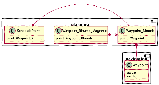
Here’s the structure of the classes in this application:

Planning Approach

Currently, the planning application computes distances and Estimated Time Enroute (ETE) for each leg. Given this information we can compute an arrival time based on a departure time.

The approach is embodied by creating a SchedulePoint object. This is direct enrichment of the Waypoint instances along the route.

Here’s how the solution is based on source data.

1. A route can be understood as a sequence of \(n\) waypoints.

   \[r_w = \langle w_0, w_1, w_2, ..., w_{n-1} \rangle\]

2. A waypoint is a latitutde (\(\phi\)), and longitude (\(\lambda\)) pair.

   \[w = \langle \phi, \lambda \rangle\]

3. A route can also be understood as a sequence of legs, \(l_i(f, t)\), formed from pairs of waypoints, called “from” and “to”. Note that we provide a placeholder leg, \(l_{n-1}\), so that each waypoint, \(w_x\), is the “from” item of a leg, \(l_x(w_x, w_{x+1} \cup \bot)\).

   \[r_l = \langle l_0(w_0, w_1), l_1(w_1, w_2), ..., l_i(w_i, w_{i+1}), ..., l_{n-2}(w_{n-2}, w_{n-1}), l_{n-1}(w_{n-1}, \bot) \rangle\]

3. The distance, \(d(f, t)\), and bearing, \(\theta(f, t)\), are computed from legs, which are pairs of waypoints. We prefer nautical miles as the units.

   \[\begin{split}d(l_i) = r(l_i \cdot f, l_i \cdot t) = r(w_i, w_{i+1}) \\ \theta(l_i) = \theta(l_i \cdot f, l_i \cdot t) = \theta(w_i, w_{i+1})\end{split}\]

4. Given speed, \(s\), in knots, we can compute ETE for each leg, \(e(l_i; s)\). This is a duration generally in hours. It’s often more useful in minutes than hours.

   \[e(l_i; s) = 60 \frac{d(l_i)}{s}\]

We often summarize the ETE to a point, \(i\), on the route. If \(i = n\), then, this is the total elapsed time enroute.

\[\sum\limits_{0 \leq x < i}e(l_x; s) = \frac{\sum\limits_{0 \leq x < i}d(l_x)}{s}\]

There are three summary computations:

• Final Arrival Time, given speed, and Departure Time. \(A_n(r; s, T_0)\).

• Initial Departure Time, given Arrival Time and speed. \(D_0(r; s, T_n)\).

• Speed, given Initial Departure Time and Final Arrival Time. \(s(r; T_0, T_n)\).

We’ll look at arrival time, first.

1. Given speed, \(s\), in knots, and a departure time, \(T_0\), we can compute ETA’s, \(A(l_i; s, T_0)\), for each leg. These are date-time stamps. We formulate this to show how it accumulates and the final result.

   \[\begin{split}A(l_i; s, T_0) &= T_0 + e(l_i; s) + \left(\sum\limits_{0 \leq x < i}e(l_x; s)\right) \\ &= T_0 + \left( \frac{\sum\limits_{0 \leq x \leq i}d(l_x)}{s} \right)\end{split}\]

2. The final arrival time, \(A_n\), then, is the last arrival time for the route, r,

   \[A_n(r; s, T_0) = A(l_n; s, T_0)\]

We can also do the computation in the reverse direction to compute departure times, \(D(l_i; s, T_n)\) to work out the departure for leg \(l_i\) required to have final arrival time T_n. We can use this to work out the initial departure time, \(D_0(r; s, T_n)\).

1. Given speed, \(s\), in knots, and an arrival time, \(T_n\), we can compute ETD’s, \(D(l_i; s, T_n)\), for each preceeding leg.

   \[\begin{split}D(l_i; s, T_n) &= T_n - e(l_i; s) - \left(\sum\limits_{0 \leq x < i}e(l_x; s)\right) \\ &= T_n - \left( \frac{\sum\limits_{0 \leq x \leq i}d(l_x)}{s} \right)\end{split}\]

2. The initial departure time, \(D_0\), then, is the first departure time for the route, r,

   \[D_0(r; s, T_n) = D(l_0; s, T_n)\]

Speed for a route, \(r\), given departure, \(T_0\), and arrival, \(T_n\).

\[s(r; T_0, T_n) = \frac{\sum\limits_{0 \leq i < n}d(l_i)}{T_n-T_0}\]

Improvements

There are a number of potential improvements to this approach:

• Include an estimated time of departure (ETD) as a basis for computing ETE and ETA.

• Include the position of the sun for each ETA.

• Include a Noon position on any leg that spans local noon.

The goal is to match the output content of opencpn_table:

• waypoint: Waypoint

• leg: int

• ETE: Optional[“Duration”]

• ETA: Optional[datetime.datetime]

• ETA_summary: Optional[str]

• speed: float

• tide: Optional[str]

• distance: Optional[float]

• bearing: Optional[float]

• course: Optional[float] = None

Improvements

There are several improvements required.

Time-of-Day

Todo

Locate the sunrise equation and include anticipated time-of-day for an ETA

See https://gml.noaa.gov/grad/solcalc/solareqns.PDF

Noon Location

Todo

Compute the locations at noon of each day.

This requires looking at waypoints before and after local noon, Splitting the segment to find noon, and adding a waypoint with no course change.

A route is a sequence of waypoints forming legs. One leg, \(l_a(w_a, w_{a+1})\), spans noon, \(N\).

We can think of arrival time and departure for this leg.

\[\begin{split}T_a = A(l_a; s, T_0) \\ T_{a+1} = A(l_{a+1}; s, T_0)\end{split}\]

\[T_a \leq N \leq T_{a+1}\]

There are three cases here, two of which are trivial. If \(T_a = N\) or \(N = T_{a+1}\), there’s no further computation required. The interesting case, then, is \(T_a < N < T_{a+1}\).

We know the distance for this leg, \(d(l_a)\). This gives us time enroute, \(e(l_a; s)\), to traverse the leg, given a speed, \(s\).

\[e(l_a; s) = \frac{d(l_a)}{s}\]

The time until noon, \(N - T_a\), is a fraction of the overall elapsed time of the leg, \(e(l_a; s)\). Which gives us distance until noon for a given leg, at a tiven speed, \(N_d(l_a; s)\),

\[\frac{N - T_a}{e(l_a; s)} = \frac{N_d(l_a; s)}{d(l_a)}\]

or,

\[N_d(l_a; s) = \frac{d(l_a)[N - T_a]}{\frac{d(l_a)}{s}} = s[N - T_a]\]

We can then offset from point \(w_a\) by distance \(N_d(la;s)\) in direction \(\theta(l_a)\) to compute the noon location. This is the navigation.destination() function.

The destination function, \(D( w, d, \theta )\), is defined like this.

\[ \begin{align}\begin{aligned}\begin{split}D_{\phi}( w, d, \theta ), &\text{ latitude at distance $d$, angle $\theta$ from $w$}\\ D_{\lambda}( w, d, \theta ), &\text{ longitude at distance $d$, angle $\theta$ from $w$}\end{split}\\D( w, d, \theta ) = \langle D_{\phi}( w, d, \theta ), D_{\lambda}( w, d, \theta ) \rangle\end{aligned}\end{align} \]

The definition of these two functions are in Destination Calculation.

Forward and Reverse Plans

Currently, only forward plans are supported.

An event more sophisticated planner would allow for all three kinds of plans:

• A “forward” plan uses a Scheduled Time of Departure (STD) to compute a sequence of ETE and ETA’s.

• A “reverse” plan would use a Scheduled Time of Arrival (STA) and work backwords to compute departures and times enroute. This would lead to a Scheduled Time of Departure (STD).

• A “speed” plan would compute optimal speed to pass between given STD and STA.

• We can also imagine pinning specific waypoints to specific STA or STD to compute variant speeds along a route.

The idea is to reduce the amount of work done with a spreadsheet outside navtools.

Implementation

This module includes several groups of components.

• The Input Parsing group is the functions and classes that acquire input from the GPX or CSV file.

• The Planning Computations functions work out range and bearing, magnetic bearing, total distance run, and elapsed time in minutes and hours.

• The Output Writing group is the functions to write the CSV result.

• Finally, the Command-Line Interface components are used to build a proper command-line application.

Input Parsing

The purpose of input parsing is to create Waypoint objects from input file sources.

A Waypoint is a 5-tuple of name, latitude, longitude, description and “point” information. The “point” information is a navigation.LatLon instance that combines the source lat and lon values.

The input parsing supports two formats: CSV and GPX. Each source format has a different kind of parser. The CSV parser uses the csv module. The GPX parser uses xml.etree; it uses the findall() method to iterate through all of the rows.

Note that the GPSNavX output was encoded in Western (Mac OS Roman). This can make CSV parsing a bit more complex because there will be Unicode characters that the CSV module doesn’t always handle gracefully. However, the patterns used for parsing tolerate the extraneous bytes that appear in the midst of degree-minute values.

navtools.planning.csv_to_Waypoint(source: TextIO) → Iterator[navtools.navigation.Waypoint]

Parses the CSV files produced by tools like GPSNavX or iNavX to yield an iterable sequence of Waypoint objects. These files had no heading row. The assumed column order is “name”, “lat”, “lon”, “description”.

Note that the old GPSNavX output was encoded in Western (Mac OS Roman). This can make CSV parsing a bit more complex because there will be Unicode characters that the CSV module doesn’t always handle gracefully. However, the patterns used for parsing tolerate the extraneous bytes that appear in the midst of degree-minute values.

Parameters

source – Open file or file-like object that can be read

Returns

iterable sequence of Waypoint instances.

navtools.planning.gpx_to_Waypoint(source: TextIO) → Iterator[navtools.navigation.Waypoint]

Generates Waypoint onjects from a GPX doc.

We assume a minimal schema:

• <rte> contains

  • <rtept lat="" lon=""> contains

    • <name>

    • <description>

In some cases, there are additional attributes available, but we don’t seem to need them for planning.

Parameters

source – an open GPX file.

Returns

An iterator over Waypoint objects.

Planning Computations

The various navigation calculations use an immutable object (or functional programming) style. A series of functions create new, richer objects from the initial Waypoint objects.

Specifically, we use the following kind of function composition.

Schedule Details

class navtools.planning.SchedulePoint(point: navtools.navigation.Waypoint, distance: float, true_bearing: Optional[navtools.navigation.Angle], magnetic: Optional[navtools.navigation.Angle], speed: Optional[float], enroute_min: Optional[float], next_course: Optional[navtools.navigation.Angle], arrival: Optional[datetime.datetime])

Scheduled waypoints. These include distance, bearing, and estimated time enroute (ETE).

Todo

Unify with opencpn_table.Leg.

• leg: int

• ETE: Optional[“Duration”]

• ETA: Optional[datetime.datetime]

• ETA_summary: Optional[str]

• speed: float

• tide: Optional[str]

• distance: Optional[float]

• bearing: Optional[float]

• course: Optional[float] = None

point: navtools.navigation.Waypoint

distance: float

true_bearing: Optional[navtools.navigation.Angle]

magnetic: Optional[navtools.navigation.Angle]

speed: Optional[float]

enroute_min: Optional[float]

next_course: Optional[navtools.navigation.Angle]

arrival: Optional[datetime.datetime]

navtools.planning.gen_schedule(waypoints: Iterable[navtools.navigation.Waypoint], variance: Callable[[navtools.navigation.LatLon, Optional[datetime.date]], float], start_datetime: Optional[datetime.datetime] = None, speed: float = 5.0) → Iterator[navtools.planning.SchedulePoint]

Calculates distance, bearing, and time en route for each waypoint. This is the forward algorithm starting from start_datetime.

The algorithm peeks ahead to compute the course to the next waypoint. This requires a route with two or more waypoints.

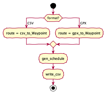
It works like this:

• Set previous = next(iter); here = next(iter)

• Yield previous with no ETE or distance, course from previous to here.

• For end in iter:

  • Compute ETE and distance from previous to here

  • Yield here with ETE and distance from previous to here and course from here to end.

  • Set previous, here = here, end; with some cleverness, we should be able to reuse distance and bearing.

• Compute ETE and distance from previous to here

• Yield here with ETE and course from previous to here and no course.

This requires a wee bit of optimization to prevent duplicate cade. We should, specifically, cache the distance and bearing to avoid recomputation.

Parameters

• waypoints – Iterable collection of Waypoint objects.

• variance – the magnetic variance (a/k/a declination) function; generally use navigation.declination().

• start_datetime – the date on which to compute the variance; default is today

• speed – Default speed assumption to use; default is 5.0 knots.

Returns

iterator over SchedulePoint instances.

Output Writing

Writes a sequence of Schedule objects to a given target file.

The file will have the following columns:

“Name”, “Lat”, “Lon”, “Desc”, “Distance (nm)”, “True Bearing”, “Magnetic Bearing”, “Distance Run”, “Elapsed HH:MM”

Note that we apply some rounding rules to these values before writing them to a CSV file. The distances are rounded to \(10^{-5}\) which is about an inch, or 2 cm more accurate than the GPS position. The bearing is rounded to zero places.

Note

It’s hard to steer to a given degree, much less a fraction of a degree. Classically, the mariner’s compass divides the circle into 32 points; this is 12.5 degrees each point. That’s an appropriate rounding for coastal cruising.

The width of your fist at arm’s length is 10°. If you extend index finger and pinky, that’s 15°. In the middle is all the accuracy you have when steering by hand.

navtools.planning.nround(value: Optional[float], digits: int) → Optional[float]

Returns a rounded value, properly honoring None objects.

Parameters

• value – Float value (or None)

• digits – number of digits

Returns

rounded float value (or None)

navtools.planning.write_csv(target: TextIO, sched_iter: Iterable[navtools.planning.SchedulePoint]) → None

Writes a sequence of Schedule objects to a given target file.

The file has the following columns:

"Name", "Lat", "Lon", "Desc",
"Distance (nm)", "True Bearing", "Magnetic Bearing",
"Distance Run", "Elapsed HH:MM"

It makes sense to unify the output with OpenCPN’s plan. This leads to the following columns:

"Leg" -- sequence number of legs.
"To waypoint" -- Waypoint name from the GPX source
"Distance" -- Equirectangular distance to the waypoint.
"True Bearing" -- True-North Bearting
"Bearing" -- Magnetic bearing (with decliation.)
"Latitude" -- Waypoint latitude from the GPX source
"Longitude" -- Waypoint longitude from the GPX source
"ETE" -- Estimated Time Enroute in "d h m" duration format.
"ETA" -- Estimated time of arrival as "date hh:mm (summary)"
"Speed" -- Given speed for this leg (usually it's all one assumed speed.)
"Next tide event" -- usually empty
"Description" -- Waypoint description from the GPX source
"Course" -- Course to steer to the next waypoint

Note that we apply some rounding rules to some values before writing them to a CSV file. The distances are rounded to \(10^{-1}\) which is about 607’. The bearing is rounded to zero places.

Parameters

• target – Open file (or file-like object) to which csv data will be written.

• sched_iter – iterator over SchedulePoint instances. For example, the output from the gen_schedule() function.

Command-Line Interface

Typical use cases for this module include the following.

• Run from the command line:

  python -m navtools.planning -s 5.0 '../../Sailing/Cruising Plans/Lewes 2011/Jackson Creek to Cape Henlopen -- Offshore.gpx'
  

• Run within a Python script:

  from navtools.planning import plan
  from pathlib import Path
  routes = Path("/path/to/routes")
  plan(routes/'Whitby Rendezvous.csv', 5.0)
  plan(routes/'Whitby Rendezvous.gpx', 5.0)
  

The plan() application

navtools.planning.plan(route_path: pathlib.Path, speed: float = 5.0, departure: Optional[datetime.datetime] = None, variance: Optional[Callable[[navtools.navigation.LatLon, Optional[datetime.date]], float]] = None) → None

Transforms a simple route into a route with a detailed schedule.

This doesn’t compute ETA’s. It computes ETE’s for each leg, and an assumed start time can be plugged in to create ETA’s.

The date is used to compute variance, but not to compute ETA’s.

Parameters

• route_filename – Source route, extracted into CSV format.

• speed – Assumed speed; default is 5.0kn.

• date – Assumed date for magnetic declination; default is today.

• variance – Declination function to use. Default is navigation.declination()

Todo

Implement arrival-based planning to solve for departure.

Todo

Implement departure and arrival planning to solve for speed.

The main() CLI

navtools.planning.main(argv: list) → None

Parses command-line arguments to get the routes file names, and the default speed to use.

Then use plan() to process each file, creating a name Schedule.csv output file with the detailed schedule.