Using Stingray Reader

We use Stingray to work with data files where the schema is either external or complex (or both). The tool lets us tackle this question:

How do we process a file simply and consistently?

In some cases, we can extend this to a more comprehensive question:

How do we make a program independent of Physical Format and Logical Layout?

We can also use Stingray to answer questions about files, the schema those files purport to use, and the data in those files. Specifically, we can tackle this question:

How do we ensure that a file and an application use the same schema?

There are two sides to this “using the same schema?” question:

• Data Quality. Does the file match the required schema?

• Software Quality. Will this application process a file with the required schema?

An underlying assumption is the schema is correct. Files or applications may not match the schema, but the schema is the standard.

We also need to note the following.

If it was simple, we wouldn’t need this package, would we?

Concepts

Here are the three levels of schema that describe the data in a file:

• Physical Format. This defines how to unpack bytes into Python objects (e.g., decode a string to lines of text to atomic fields). We want to make this transparent to our applications, so we can focus on the data and the processing. When using Stingray, everything is a workbook with sheets, rows, cells, and a consistent API.

• Logical Layout. This defines how to locate the values within row structures that may not have perfectly consistent column order. Sometimes the Logical Layout is described by a schema embedded in the file: it might be the top row of a sheet in a workbook, for example. Sometimes the logical layout can be in a separate file: a COBOL data definition, or perhaps a metadata sheet in a workbook.

• Conceptual Content. A single conceptual schema of has data represented by a number of logical layouts. Sometimes the data is represented in a number of physical formats. An application should be able to tolerate variability as long is the data reflects a consistent conceptual content.

We can’t make the logical layout of data completely transparent to the application programs. The column names in the metadata, at a bare minimum, are a visible aspect of the layout. The order or position of the columns in each row, however, need not be fixed.

Since we’re working in Python, the conceptual schema is often defined by an application’s class definitions. The idea is to support ways to build class instances that are tolerant of variations in the logical layout. This should also be independent of physical format.

The unifying theme is to have a conceptual schema. This schema then supports application processing without regard to layout and format.

Schema-Based Processing

All Stingray applications involve two elements:

• a source of data, a Workbook object,

• and a schema, an instance of the Schema class.

Here are the essential relationships among the concepts:

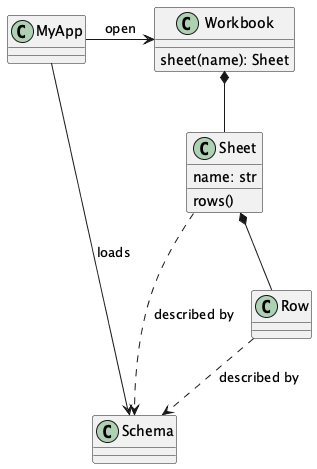
The schema can originate in a variety of places:

• A Schema can be the first row of a spreadsheet. Think of the csv.DictReader class, which examines the given file for a header row, creates a minimal schema from this row, and uses the schema to unpack the remaining rows.

• A Schema can be in a separate document. There are a number of choices.

  • For COBOL files, the schema is a “Copybook” with the COBOL Data Definition Entry (DDE) for the file. The schema is COBOL code.

  • A sheet of a workbook may have “metadata” with column definitions. This is a schema represented as a workbook. The columns of this metadata sheet have a metaschema.

• A JSON Schema can be embedded in the code. Ideally, it’s in a separate module that can be shared by many applications. The sharing assures consistent Conceptual Content among applications.

There are, in effect, four use cases for gathering schema that can be used to process data.

This leads us to four patterns for working with Schema to access data. We’ll look at each of them in the next section.

Essential Patterns of Schema Use

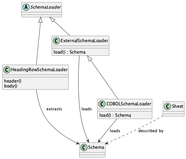
There are four patterns to loading the schema before working with the data:

• The schema is in one (or more) header rows of a sheet in a workbook.

• The schema is in an external file, i.e., another workbook, or another sheet in the data workbook.

• The schema is defined by a COBOL DDE in a “copybook”. This is an external file, but with more complex syntax, not another workbook with a distinct metaschema.

• A schema is embedded in the application as class definitions or JSON Schema documents.

We’ll look at each in some detail.

Schema in Header Rows

When the header row has a schema, the processing is vaguely similar to working with the csv module. There are two steps to processing the data.

1. Load the schema from the first row.

2. Process the remaining rows using the loaded schema.

For CSV, COBOL, and similar structures, there is a single conceptual sheet in the workbook. This one-and-only sheet is named "". Rather than assume a default sheet with this name, Stingray requires an explicit reference to the sheet named "".

The header row processing looks like this:

>>> from stingray import open_workbook, HeadingRowSchemaLoader, Row
>>> from pathlib import Path
>>> import os
>>> from typing import Iterable

>>> def process_rows(rows: Iterable[Row]) -> None:
...     for row in rows:
...         print(row.name("x123").value(), row.name("y1").value())

>>> data_path = Path(os.environ.get("SAMPLES", "sample")) / "Anscombe_quartet_data.csv"
>>> with open_workbook(data_path) as workbook:
...    sheet = workbook.sheet("")
...    _ = sheet.set_schema_loader(HeadingRowSchemaLoader())
...    process_rows(sheet.rows())
10.0 8.04
8.0 6.95
13.0 7.58
9.0 8.81
11.0 8.33
14.0 9.96
6.0 7.24
4.0 4.26
12.0 10.84
7.0 4.82
5.0 5.68

The essential processing, in the process_rows() function, uses the Row class. Each Row instance has columns.

The HeadingRowSchemaLoader built a schema from the header row. This is a stripped-down-to-almost-nothing schema with column names and default data types of string. The schema derived from a CSV header – by itself – only has column names. The schema could provide additional information, like data conversions to perform for each column.

Schema in an External File

For an external schema, here are the two steps to processing the data:

1. Load the schema. This involves opening a workbook that has the schema, This external schema has its own metaschema, ideally as header rows.

2. Process data using the loaded schema.

External schema processing look like this:

>>> from stingray import open_workbook, ExternalSchemaLoader, Row, SchemaMaker
>>> from pathlib import Path
>>> import os
>>> from typing import Iterable

>>> def process_rows(rows: Iterable[Row]) -> None:
...     for row in rows:
...         print(row.name("x123").value(), row.name("y1").value())

1. Load the Schema by reading a CSV file
>>> schema_path = Path(os.environ.get("SAMPLES", "sample")) / "Anscombe_schema.csv"
>>> with open_workbook(schema_path) as metaschema_workbook:
...     schema_sheet = metaschema_workbook.sheet("Sheet1")
...     metaschema = SchemaMaker().from_json(ExternalSchemaLoader.META_SCHEMA)
...     _ = schema_sheet.set_schema(metaschema)
...     json_schema = ExternalSchemaLoader(schema_sheet).load()
>>> schema = SchemaMaker().from_json(json_schema)

2. Process the rows using the schema
>>> data_path = Path(os.environ.get("SAMPLES", "sample")) / "Anscombe_quartet_data.csv"
>>> with open_workbook(data_path) as workbook:
...     sheet = workbook.sheet("").set_schema(schema)
...     process_rows(sheet.rows())
x123 y1
10.0 8.04
8.0 6.95
13.0 7.58
9.0 8.81
11.0 8.33
14.0 9.96
6.0 7.24
4.0 4.26
12.0 10.84
7.0 4.82
5.0 5.68

The first step – reading the external schema – involves opening a schema workbook, and preparing to read the schema sheet. What’s on this schema definition sheet? In this example, we’ve used the ExternalSchemaLoader.META_SCHEMA to define the columns of the schema.

If no metaschema is defined by the set_schema() method, a HeadingRowSchemaLoader is used. This will use column names in the first row of the schema sheet.

The ExternalSchemaLoader builds a schema from a sheet that must provide column names, column data conversions, and a column description. The metaschema must match the following JSON Schema definition:

{
    "title": "generic meta schema for external schema documents",
    "type": "object",
    "properties": {
        "name": {"type": "string", "description": "field name", "position": 0},
        "description": {
            "type": "string",
            "description": "field description",
            "position": 1,
        },
        "dataType": {
            "type": "string",
            "description": "field data type",
            "position": 2,
        },
    },
}

Three columns are required by this definition:

• name

• description

• dataType

If your schema doesn’t look like this, you’ll need to define a metaschema, similar to the JSON Schema document shown here.

Once the the external schema has been loaded, it is used to process the target data. The process_rows() function can consume rows with the attribute names and types that are defined in the external Anscombe_schema.csv file. Because of the schema, automated conversions from strings to float can be done by Stingray.

An essential feature of this is the processing does not change, even though the source data physical format and logical layout can change. Further, it becomes possible to tolerate a variety of schema definition alternatives.

Schema in a COBOL Copybook

COBOL Processing is similar to external schema loading. First, the application loads the schema from the COBOL copybook file. Then, the application can process data using the schema.

COBOL processing looks like this:

>>> from stingray import schema_iter, COBOL_Text_File
>>> from pathlib import Path
>>> import os

>>> def process_rows(rows: Iterable[Row]) -> None:
...     for row in rows:
...         print(row.name("X123").value(), row.name("Y1").value())

1. Load the Schema by reading a COBOL CPY file
>>> copybook_path = Path(os.environ.get("SAMPLES", "sample")) / "anscombe.cpy"
>>> with copybook_path.open() as source:
...     schema_list = list(schema_iter(source))
>>> json_schema, = schema_list  # Take the first; ignore any other 01-level records
>>> schema = SchemaMaker().from_json(json_schema)

2. Process the rows using the schema
>>> data_path = Path(os.environ.get("SAMPLES", "sample")) / "anscombe.data"
>>> with COBOL_Text_File(data_path) as workbook:
...     sheet = workbook.sheet('').set_schema(schema)
...     process_rows(sheet.rows())
 010.00  008.04
 008.00  006.95
 013.00  007.58
 009.00  008.81
 011.00  008.33
 014.00  009.96
 006.00  007.24
 004.00  004.26
 012.00  010.84
 007.00  004.82
 005.00  005.68

The schema_iter() function reads all of the COBOL record definitions in the given file. While it’s common to have a single “01-level” layout in a file, this isn’t universally true. The parser will examine all of the record definitions. In the cases where there’s a single definition, the result will be a list with only one item.

The process_rows() function for working with COBOL is nearly identical to the previous two examples. The column names x123 and y1 are switched to upper case, which is a little more typical of COBOL.

The COBOL definition for this file is the following:

01  ANSCOMBE.
    05  X123   PIC S999.99.
    05  FILLER PIC X.
    05  Y1     PIC S999.99.
    05  FILLER PIC X.
    05  Y2     PIC S999.99.
    05  FILLER PIC X.
    05  Y3     PIC S999.99.
    05  FILLER PIC X.
    05  X4     PIC S999.99.
    05  FILLER PIC X.
    05  Y4     PIC S999.99.

The attributes all use a “USAGE DISPLAY” format, which makes them string values. Any conversion to a number becomes part of the application processing. This is a consequence of sticking closely to COBOL semantics for the the data definitions.

Schema In the Application

A Schema can be built within the application, also. This can be done using Stingray‘s internal data structures. However, it seems simpler to use JSON Schema as a starting point, and build the internal structure from the JSON Schema document.

>>> from stingray import open_workbook, ExternalSchemaLoader, Row, SchemaMaker
>>> from pathlib import Path
>>> import os
>>> from typing import Iterable

>>> def process_rows(rows: Iterable[Row]) -> None:
...     for row in rows:
...         print(row.name("x123").value(), row.name("y1").value())

1. Load a literal schema

   >>> json_schema = {
   ...     "title": "spike/Anscombe_quartet_data.csv",
   ...     "description": "Four series, use (x123, y1), (x123, y2), (x123, y3) or (x4, y4)",
   ...     "type": "object",
   ...     "properties": {
   ...         "x123": {
   ...             "title": "x123",
   ...             "type": "number",
   ...             "description": "X values for series 1, 2, and 3.",
   ...         },
   ...         "y1": {"title": "y1", "type": "number", "description": "Y value for series 1."},
   ...         "y2": {"title": "y2", "type": "number", "description": "Y value for series 2."},
   ...         "y3": {"title": "y3", "type": "number", "description": "Y value for series 3."},
   ...         "x4": {"title": "x4", "type": "number", "description": "X value for series 4."},
   ...         "y4": {"title": "y4", "type": "number", "description": "Y value for series 4."},
   ...     },
   ... }
   >>> schema = SchemaMaker().from_json(json_schema)
   

2. Process the rows using the schema

   >>> data_path = Path(os.environ.get("SAMPLES", "sample")) / "Anscombe_quartet_data.csv"
   >>> with open_workbook(data_path) as workbook:
   ...     sheet = workbook.sheet('').set_schema(schema)
   ...     process_rows(sheet.rows())
   x123 y1
   10.0 8.04
   8.0 6.95
   13.0 7.58
   9.0 8.81
   11.0 8.33
   14.0 9.96
   6.0 7.24
   4.0 4.26
   12.0 10.84
   7.0 4.82
   5.0 5.68
   

The JSON Schema description is relatively clear, and easy to write as a Python dictionary literal. This representation can be shared widely among multiple applications. This could be part of an OpenAPI specification, for example, shared by a RESTful web server with the client applications.

Rows and Navigation

A Row is a binding between an instance of raw data from the underlying COBOL file or workbook structure, and a schema.

Most workbook rows are a flat sequence of named columns. The JSON Schema definition is an “object”; each column is a property. For COBOL, a simple list of columns isn’t appropriate. For delimited files (i.e., NDJSON, YAML, or TOML) a flat list of names isn’t appropriate, either.

To unify all of these, a Row object uses a navigation aid. These are Nav instances that are used to locate the proper strings of bytes.

Ordinarily, the Nav objects are invisible. When an application uses an expression like row.name("name").value(), this will extract a Python object that is the value. An intermediate Nav object will be created, but it is not visible.

A Nav object can be visible when we omit the Nav.value method. This extracts the final Python object from the cell. It may be useful to cache Nav objects to improve performance.

Here’s the relationship:

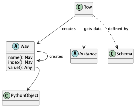
The Instance is a union of the various kinds of instance extraction protocols: NDInstance, DInstance, and WBInstance. These handle the non-delimited files (i.e. COBOL, and similar), delimited files, and spreadsheet workbooks. An Instance has methods to get items by name or by column number from the underlying file or workbook.

The fluent interface of a Nav will create additional Nav navigation helpers to work down into a complex structure. This is particularl important for COBOL.

Generally, COBOL programs assume all field names are unique. (They don’t have to be, but this is rare.) To make this work out well, Stringray leverages JSON Schema $anchor keywords to avoid complex path-based navigation into an object. Using anchor names allows a Nav.name() method to locate a field deeply nested inside a complex COBOL record. The parallels the way the COBOL language works.

Application Design Considerations

We’ll cover several more examples of schema-based processing. It’s important to design an application around data quality and software quality considerations.

More examples are in the demonstration applications shown in the Demo Applications section.

All schemae start as JSON Schema documents. These are Python dict[str, Any] structures. A stingray.workbook.SchemaMaker object is used to transform the JSON Schema document into a usable stingray.schema_instance.Schema object. This permits pre-processing the schema to add features or correct problems.

This use of JSON Schema assures that schema can be loaded from a wide variety of sources and are compatible with a wide variety of other software tools.

Data Capture and Builder Functions

There are two parts to data handling: Capture and Conversion. Data processing starts with Capture. Using a schema is the heart of solving the semantic problem of capturing data in spreadsheet and COBOL files. We’ll look at Capture in this section, and then Conversion in the next section.

We want to have just one application that is adaptable to a number of variant logical layouts. These must reflect alternative implementations of a single conceptual content. Ideally, there’s one layout and one schema, but as a practical matter, there are often several similar schemae.

We need to provide three pieces of information for capture:

• Target variable (or attribute or parameter) used by our application.

• Target data type needed by our application.

• Source navigation based on attribute name or position in the source file. In the case of COBOL or JSON with deeply nested structures, this navigation can be complex. In the case of a CSV, it’s a name or column number.

This triple is essentially a Python assignment statement with target, to_type and source. A DSL or other encoding is unhelpful.

A simple description is the following:

target = to_type(row['source'].value())

There is a tiny bit of boilerplate in this assignment statement. The overhead of the boilerplate is offset by the flexibility of using Python directly.

We can use either schema.name('source') or schema['source'] as a way to locate a named attribute within a schema.

There are some common cases that will extend or modify the boilerplate. In particular, COBOL structures that are not in first normal form will include array indexing. COBOL can have ambiguous names, requiring a navigation path to an atomic value. Finally, because of the COBOL redefines feature, it helps to do lazy evaluation to compute the value after navgiating to the desired string of bytes.

This is our preferred design pattern: a Builder Function:

def build_record_dict(aRow: Row) -> dict[str, Any]:
    return dict(
        name = row['some column'].value(),
        address = row['another column'].value(),
        zip = digits_5(row['zip'].value),
        phone = row['phone'].value(),
    )

This function defines the application-specific mapping from a row in a source file. It leverages logical layout information from the schema definition.

Of course, the schema can lie, and the application can misuse the data. Those are inevitable (and therefore insoluble) problems. This is why we must write customized software to handle these data sources.

In the case of variant schemae, we can use something like this.

def build_record_dict_1(aRow: Row) -> dict[str, Any]:
    return dict(
        name = row['some column'].value(),
        address = row['another column'].value(),
        zip = digits_5(row['zip'].value()),
        phone = row['phone'].value(),
    )

def build_record_dict_2(aRow: Row) -> dict[str, Any]:
    return dict(
        name = row['variant column'].value(),
        address = row['something different'].value(),
        zip = digits_5(row['zip'].value()),
        phone = row['phone'].value(),
    )

We can then define a handy factory which picks a builder based on the schema version.

def make_builder(args: argparse.namespace) -> Callable[[Row], dict[str, Any]]:
    return eval('build_record_dict_{args.layout}')

Some people worry that an Evil Super-Genius (ESG) might somehow try to exploit the eval() function. The ESG would have to be both clever and utterly unaware that the source is easily edited Python People who worry about an ESG that can manipulate the parameters while unable to simply edit the Python can use the following:

{'1': build_record_dict_1, '2': build_record_dict_2}[args.layout]

The make_builder() function selects one of the available builders based on a command-line option in the args structure.

Data Conversions

There are two parts to data handling: Capture and Conversion. Conversion is part of the final application, once the source data has been captured.

A target data conversion can be rather complex. It can involve involve any combination of filtering, cleansing, conforming to an existing database, or rewriting.

Here’s a much more complex Builder Function that includes conversion.

def build_record_3(aRow: Row) -> dict[str, Any]:
    if not aRow['flag']:
        return {}
    zip_str = aRow['zip'].value()
    if '-' in zip:
        zip = digits_9(zip_str.replace('-', ''))
    else:
        if len(zip) <= 5:
            zip = digits_5(zip_str)
        else:
            zip = digits_9(zip_str)
    return dict(
        name = aRow['variant column'].value(),
        address = arow['different column'].value(),
        zip = zip,
        phone = aRow['phone'].value(),
    )

This shows filtering and cleansing operations. Yes, it’s complex. Indeed, it’s complex enough that attempting to define a domain-specific language will lead to more problems than simply using Python for this.

Stingray Application Design

A application need to consider two tiers of testing. Conventional unit testing makes sure the application’s processing is valid. Beyond that, data quality testing ensures that the data itself is valid.

Data quality testing is facilitated by some specific design patterns for the application as a whole.

For application unit testing, our programs should be decomposed into three tiers of processing.

• Row-Level. Inidividual Python objects built from one row of the input. This involves our builder functions.

• Sheet-Level. Collections of Python objects built from all rows of a sheet. This involves sheet processing functions. Mocked row-level functions should be used.

• Workbook-Level. In some cases, we may need to work with a collection of sheets. If required, these tests will need mocked sheet and row functions.

Each of these tiers should be tested independently.

For data quality testing, we need to validate that the the input files meet the expected schema. This can use the unit testing framework. However, it’s often more helpful to design application software to work in a “dry-run” or “validation” mode. This operating mode can check the data without make persistent state changes to other files or databases.

Row-Level Processing

Row-level processing is centered on the builder functions. These handle the detailed mapping from variant logical layouts to a single conceptual schema.

A builder function can create a simple dictionary. Note that there are two separate steps:

• Preparing data for a candidate object. A dict[str, Any] has data values. There may be a number of different builder functions for this.

• Building an application object from candidate data. These objects are often a typing.NamedTuple or dataclasses.dataclass. These should not vary with the logical layout.

This design echoes the design patterns from the Django project, where a ModelForm is used to validate data before attempting to build a Model instance.

An alternative is to follow the design patterns of the Pydantic project, where validation is bundled into the class definition. Using pydantic data class definitions can slightly simplify these examples by bundling validation into the model class.

Validation within the class __init__() method, while possible, is often awkwardly complex. There are two separate things bound together: validating and initialization. While these can be separated into methods used by __init__(), each change to a logical layout becomes yet another subclass. In this case, composition seems more flexible than inheritance.

One additional reason for decomposing the building from the application object construction is to support multiprocessing pipelines. It’s often quicker to serialize a Python object built as dict[str, Any] than to serialize an instance of a new class.

Here’s the three-part operation: Build, Validate, and Construct.

def builder_1(row: Row) -> dict[str, Any]:
    return dict(
        key = row['field'].vaue(),
    )

def is_valid(row_dict: dict[str, Any]) -> bool:
    All present or accounted for?
    return state

def construct_object(row_dict: dict[str, Any]) -> App_Object:
    return App_Object(**row_dict)

The validation rules rarely change. The object construction doesn’t always need to be a separate function, it can often be a simple class name, or a classmethod of the class.

Our sheet processing can include a function like this:

builder = make_builder(args)
for row in sheet:
    intermediate = builder(row)
    if is_valid(intermediate):
        yield construct_object(intermediate)
    else:
        log.error(row)

The builder() function allows processing to vary with the file’s actual schema. We need to pick the builder based on a “logical layout” command-line option. Something like the following is used to make an application flexible with respect to layout.

def make_builder(args: argparse.Namespace) -> Callable[[Row], dict[str, Any]]:
    if args.layout in ("1", "D", "d"):
        return builder_1
    elif args.layout == "2":
        return builder_2
    else
        raise Exception(f"unknown layout value: {args.layout}")

The builders are tested individually. They are subject to considerable change. New builders are created frequently.

The validation should be common to all logical layouts. It’s not subject to much variation. The validation and object construction doesn’t have the change velocity that builders have.

Now that we can process individual rows, we need to provide a way to process the collection of rows in a single sheet.

Sheet-Level Processing

For the most part, sheets are rows of a single logcal type. In exceptional cases, a sheet may have multiple types coincedentally bound into a single sheet. We’ll return to the multiple-types-per-sheet issue below.

For the single-type-per-sheet, we have a processing function like the following:

def process_sheet(sheet: Sheet, builder: Builder = builder_1) -> Counter:
    counts = Counter()
    object_iter = (
        builder(row)
        for row in sheet.row_iter()
    )
    for source in object_iter:
        counts['read'] += 1
        if is_valid(source):
            counts['valid'] += 1
            # The real processing
            obj = make_app_object(source)
            obj.save()
        else:
            counts['invalid'] += 1
    return counts

This kind of sheet is tested two ways. First, this can have a unit test with a fixture that provides specific rows based on requirements, edge-cases and other “white-box” considerations.

Second, an integration test can be performed with live data. The counts can be checked. This actually tests the file as much as it tests the sheet processing function.

Workbook Processing

The overall processing of a given workbook input looks like this.

def process_workbook(source: Workbook, builder: Builder) -> None:
    for name in source.sheet_iter():
        # Sheet filter?  Or multi-way elif switch?
        sheet = source.sheet(name).set_schema_loader(HeadingRowSchemaLoader)
        counts = process_sheet(sheet, builder)
        pprint.pprint(counts)

This makes two claims about the workbook.

• All sheets in the workbook have the same schema rules. In this example, it’s an embedded schema in each sheet and the schema is the heading row.

• A single process_sheet() function is appropriate for all sheets.

If a workbook doesn’t meet these criteria, then a (potentially) more complex workbook processing function is needed. A sheet filter is usually necessary.

Sheet name filtering is also subject to the kind of change that builders are subject to. Each variant logical layout may also have a variation in sheet names. It helps to separate the sheet filter functions in the same way builders are separated. New functions are added with remarkable regularity

def sheet_filter_1(name: str):
    return re.match(r'pattern', name)

Or, perhaps something like this that uses a shell file-name pattern instead of a more sophisticated regular expression.

def sheet_filter_2(name: str):
    return fnmatch.fnmatch(name, 'pattern')

Command-Line Interface

We should design an application to an optional argument for verbosity. It should use a positional argument that provides all the files to profile. The design often looks like the following:

def parse_args():
    parser = argparse.ArgumentParser()
    parser.add_argument('file', nargs='+')
    parser.add_argument('-l', '--layout')
    parser.add_argument('-v', '--verbose', dest='verbosity',
        default=logging.INFO, action='store_const', const=logging.DEBUG )
    return parser.parse_args()

The overall main program looks something like this.

if __name__ == "__main__":
    logging.basicConfig(stream=sys.stderr)
    args = parse_args(sys.argv[1:])
    logging.getLogger().setLevel(args.verbosity)
    builder = make_builder(args)
    try:
        for file in args:
            with workbook.open_workbook(input) as source:
                process_workbook(source, builder)
        status = 0
    except Exception as e:
        logging.exception(e)
        status = 3
    logging.shutdown()
    sys.exit(status)

This main program switch allows us to test the various functions (process_workbook(), process_sheet(), the builders, etc.) in isolation.

It also allows us to reuse these functions to build larger (and more complete) applications from smaller components.

In Demo Applications we’ll look at two demonstration applications, as well as a unit test.

Variant Records and COBOL REDEFINES

Ideally, a data source is in “first normal form”: all the rows are a single type of data. If so, we can apply a Build, Validate, Construct sequence simply.

In too many cases, a data source has multiple types of data. In COBOL files, it’s common to have header records or trailer records which are summaries of the details sandwiched in the middle.

Similarly, a spreadsheet may be populated with summary rows that must be discarded or handled separately. We might, for example, write the summary to a different destination and use it to confirm that all rows were properly processed.

Because of the COBOL REDEFINES clause, we have multiple variants within a schema. The JSON Schema oneOf keyword captures this. This means that some of the alternatives may not have a valid decoding for the bytes. This feature mandates lazy evaluation of each attribute of each row.

We’ll look at a number of techniques for handling variant records.

Trivial Filtering

When loading a schema based on headers in the sheet, the stingray.HeadingRowSchemaLoader class will be used. We can extend this loader to reject rows, also.

The stingray.HeadingRowSchemaLoader.body() method can do simple filtering. This is most appropriate for excluding blank rows or summary rows from a spreadsheet.

Multiple Passes and Filters

When we have multiple data types within a single sheet, we can process this data using the Multiple Passes and Filters pattern. Each pass through the data uses different filters to separate the various types of data.

The multiple-pass option looks like this. Each pass applies a filter and then does the appropriate processing:

def process_sheet_filter_1(sheet: Sheet):
    counts = Counter()
    for source in sheet.row_iter():
        counts['read'] += 1
        if filter_1(row):
            intermediate = builder(row)
            counts['filter_1/pass'] += 1
            processing_1(intermediate)
        else:
            counts['filter_1/reject'] += 1
    return counts

Each filter is a simple boolean function like this.

def filter_1(source: Rpw) -> bool:
    return some condition

The conditions may be small boolean expressions like source['column'].value() == value, which means a lambda object can be used. It’s generally a good practice to encapsulate them as distinct, named functions.

One Pass and Case

When we have multiple data types within a single sheet, we can make single pass over the data, using an if-elif chain or a match-case statement. Each type of row is handled separately.

The one-pass option looks like this. A “switch” function is used to discriminate each kind of row that is found in the sheet.

def process_sheet_switch(sheet: Sheet) -> Counter:
    counts = Counter(int)
    for row in sheet.row_iter():
        counts['read'] += 1
        if switch_1(row):
            intermediate_1 = builder_1(row)
            processing_1(intermediate_1)
            counts['switch_1'] += 1
        elif switch_2(row):
            intermediate_2 = builder_2(row)
            processing_2(intermediate_2)
            counts['switch_2'] += 1
        elif etc.
        else:
            counts['rejected'] += 1
    return counts

Each switch function is a simple boolean function like this.

def switch_1(row: Row) -> bool:
    return some condition

The conditions may be trivial: source['column'].value() == value.

It often makes sense to package switch, builder, and processing into a single class.

We may be able to build a mapping from switch function results to process function.

This allows us to write a sheet processing function like this>

def process_sheet_switch(sheet: Sheet) -> Counter:
    counts = Counter()
    for source in sheet.row_iter():
        counts['read'] += 1
        processed = None
        choices: list[tuple[bool, Callable[[Row], None]] = {
            (switch_1(row), builder_1, processing_1),
            (switch_2(row), builder_2, processing_2),
            ...
        )
        for switch, builder_function, processing_function in choices:
            if switch:
                processed = switch.__name__
                counts[processed] += 1
                intermediate = builder_function(row)
                processing_function(intermediate)
        if not processed:
            counts['rejected'] += 1
    return counts

This can more easily be extended by adding to the choices mapping.

More complex pipelines

In many cases, we need to inject data quality validation before attempting to build the application object. If so, that can be added to the mapping.

It can help to define a class to contain the various pieces of the processing.

class Sequence(abc.ABC):
    @abstractmethod
    def switch(self, row: Row) -> bool: ...
    @abstractmethod
    def builder(self, row: Row) -> dict[str, Any]: ...
    @abstractmethod
    def validate(self, dict[str, Any]:) -> bool: ...
    @abstractmethod
    def process(self, dict[str, Any]) -> None: ...

    def handle(self, row: Row) -> str:
        name = self.__class__.__name__
        if not self.switch(row):
            return f"{name}-reject"
        intermediate = self.builder(row)
        if not valid(intermediate):
            return f"{name}-invalid"
        self.process(intermediate)
        return f"{name}-process"

class Record_Type_1(Sequence):
    def switch(self, row: Row) -> bool:
        return some expression
    def builder(self, row: Row) -> dict[str, Any]: ...
        return {
            name = row[column].value(),
            ...
        }
    def validate(self, intermediate: dict[str, Any]) -> bool:
        return some expression
    def process(self, intermediate: dict[str, Any]) -> None:
        do something

OPTIONS = [Record_Type_1(), Record_Type_2(), ...]

This serves as the configuration for a number of processing alternatives. New classes can be added and the OPTIONS list updated to reflect the current state of the processing.

def process_sheet_switch(sheet: Sheet) -> Counter:
    counts = Counter()
    for source in sheet.row_iter():
        counts['read'] += 1
        processed = None
        for option in OPTIONS:
            outcome = option.handle(source)
            counts[outcome] += 1
    return counts

This generic sheet processing can comfortably handle complex variant row issues. It permits a single configuration via the OPTIONS sequence to handle records appropriately.

This design permits the switch conditions to overlap, potentially processing a single row multiple times. If the conditions do not overlap, then the first outcome that ends in “-process” would exit the loop.

for option in OPTIONS:
    outcome = option.handle(source)
    counts[outcome] += 1
    if outcome.endswith("-process"):
        break

With this additional feature, the order of the conditions in the OPTIONS list becomes relevant. A general, fall-back switch() method condition must be last.

Big Data Performance

We’ve broken appllication processing down into separate steps which work with generic Python data structures. This permits use of multiprocessing to spread the pipeline into separate processors or cores.

We’ll set aside the initial switch decision-making for a moment and focus on a three step Build, Vaidate, Process sequence of operations. Each stage of of this sequence can be processed concurrently.

The Build stage uses a Sheet object’ss row_iter() method to gather Row objects. These can be validated and an intermediate object created and placed into a queue for validation.

The Validate stage dequeues intermediate objects, performs the validation checks. Valid objects are placed in a queue for processing.

The Process stage dequeues intermediate objects and processes them. There can be a pool of workers doing this in case the processing is very time-consuming.

This is amenable to asyncio, also. In that case, the final processing would be a threadpool instead of a process pool. When using ayncio it’s critical to avoid updates to shared data structures. In the rare case when this is required, explicit locking will be required and can stall the async pipeline.

File Naming and External Schema

Some data management discipline is needed be sure that the schema and file match up properly. Naming conventions and standardized directory structures are essential for working with external schema.

Well Known Formats

For well-known physical formats (.csv, .xls, .xlsx, .xlsm, .ods, .numbers) the filename extension describes the physical format. Additional schema information is required to determine the Logical Layout.

The schema may be loaded from column headers, in which case the binding is handled via an embedded schema loader. If the stingray.HeadingRowSchemaLoader is used, no more information is required. If an external schema loader is used (perhaps because the headings are not part of the sheet), then we must bind each application to the appropriate external schema for a given file.

When the schema is external, the schema will often require a unique meta-schema. This means a data file must be associated with a schema file and a schema loader for the schema.

File naming rules don’t often work out for this, and some kind of explicit configuration file may be required. In some cases, the directory structure can be used to associate data files and schema files and meta-schema.

Fixed Formats and COBOL

For fixed-format files, the filename extension does not describe the physical layout. There is not widely-used extension for fixed-format files. A suffix like .dat is uninformative. Making things slightly sompler, a fixed format schema combines logical layout and physical format into a single description.

For fixed format files, the following conventions help bind a file to its schema.

• The data file suffix should be the base name of a schema file. For example, mydata.someschema points to the someschema.cob or someschema.json schema.

• Schema files must be be either JSON Schema, a COBOL DDE file, or a workbook in a well-known format. For example someschema.cob or someschema.xlsx.

Examples. We might see the following file names.

september_2001.exchange_1
november_2011.some_dde_name
october_2011.some_dde_name
exchange_1.xls
some_dde_name.cob

The september_2001.exchange_1 file is a fixed format file which requires the exchange_1.xls metadata workbook. The metadata workbook should have an easy-to-understand schema, ideally a heading row.

The november_2011.some_dde_name and october_2011.some_dde_name files are fixed format files which require the some_dde_name.cob metadata.

External Schema Workbooks

A workbook with an external schema sheet must adhere to a few conventions to be usable. These rules form the basis for the stingray.ExternalSchemaLoader class. To change the rules, extend that class.

The metaschema is defined in the class-level META_SCHEMA variable. This is a JSON Schema definition with the following properties:

• The column names “name”, “description”, “dataType” are used.

• Additional columns are allowed, but will be ignored.

• Type definitions are the JSON Schema values: “string”, “number”, “integer”, and “boolean”.

For simple column name changes, the META_SCHEMA can be replaced. For more complex changes, the class will need to be extended.

Binding a Schema to an Application

We would like to be sure that our application’s expectations for a schema are aligned with the schema actually present. An application has several ways to bind its schema information.

• Implicitly. The code simply mentions specific columns (either by name or position). If the schema definition doesn’t match the code there will be run-time KeyError exceptions.

• Explicitly. The code has a formal “requires” check to be sure that the schema provided by the input file actually matches the schema required by the application.

The idea of explicit schema parallels the configuration management issue of module dependency. A data file can be said to conform to a given schema and an application requires conformance to a given schema.

An explicit check is far from fool proof. It’s – at best – a minimal confirmation that an expected set of attributes are present.

valid = all(
    req in schema for req in ('some', 'list', 'of', 'required', 'columns')
)

This is essential when using a spreadsheets heading row as a schema.

A better approach is to have an expected schema. We can then compare the schema built by the heading row with the expected schema. A heading row schema has no data type or conversion information, making it inadequate for most applications.

valid = all(
    prop_name in found_schema.properties for prop_name in expected_schema.properties
)

This assures us that the heading row schema found in the file includes the expected schema. It may have additional columns, which will be ignored.

The more complete check is row-by-row data validation. This is often necessary. We’ll turn to data validation below.

Schema Version Numbering

JSON Schema and XSD’s can have version numbers. This is a very cool.

See http://www.xfront.com/Versioning.pdf for detailed discussion of how to represent schema version information.

Databases, however, lack version numbering in the schema. This leads to potential compatibilty issues between application programs that expect version 3 of the schema and an older database that implements version 2 of the schema.

Our file schema, similarly, don’t have a tidy, unambiguous numbering.

For external schema, we can embed the version in the file names. We might want to use something like this econometrics_vendor_1.2. This identifies the generic type of data, the source for that file, and the schema version number.

Within a SQL database, we can use the schema name to carry version information. We could have a name_version kind of convention for the database schema objects that contain our tables. This allows an application to confirm schema compatibility with a trivial SQL query.

For embedded schema in a spreadsheet, however, we have no easy way to provide schema identification and version numbering. We’re forced to build an algorithm to examine the actual names in the embedded schema to deduce the version.

This problem with embedded schema leads to using data profiling to reason out what the file is. This may devolve to a manual examination of the data profiling results to allow a human to determine the schema. Then, once the schema has been identified, command-line options can be used to bind the schema to file for correct processing.

Data Handling Special Cases

We’ll look at a number of special cases for handling bad or unusual data.

Handling Bad Data

For inexplicable reasons, we can wind up with files that are damaged in some way.

“there is a 65-byte “header” at the start of the file, what would be the best (least hacky) way to skip over the first 65 bytes?”

This is one of the reasons why use both a file name and an open file object as arguments for opening a workbook.

path = Path("file_with_junk.some_schema")
with path.open(,"rb") as cobol:
    cobol.seek(66)
    wb = stingray.COBOL_EBCDIC_File(path, file_object=cobol)

This skips past the junk.

Leading Zeroes Digit Strings – US ZIP Codes, Social Security Numbers, etc.

Spreadsheets turn US Zip codes into numbers, and the leading zeroes get lost. This happens with social security numbers, also. It’s rare with telephone numbers. Some part numbers and UUID’s may have leading zeroes that can be lost when a spreadsheet touches the values.

In all cases, these are “digit strings”. A code that’s essentially a string but the domain of characters for that string is limited to the ten decimal digits.

This also happens with JSON, YAML, and TOML files. The solution in those cases is to add quotes to force interpretation as a string. This can’t be done to workbook data.

To handle digit strings, Stingray has conversion functions like stingray.digits_5() to turn an integer into a 5-position string with leading zeroes.

Currency

Spreadsheets turn currency into floating-point numbers. Any computation can lead to horrible ‘3.9999999997’ numbers instead of ‘4.00’. This is masked by spreadsheet applications through extremely clever formatting rules that will obscure the underlying complexity of representing currency with floating-point values.

To handle currency politely, Stingray has a stingray.decimal_2() conversion function to provide a decimal value rounded to two decimal places. When this is done as early in the processing as possible, currency computations work out nicely.